How to use SBpipe
SBpipe pipelines can be executed natively or via Snakemake, a dedicated and more advanced tool for running computational pipelines.
Run SBpipe natively
SBpipe is executed via the command sbpipe. The syntax for this command and its complete list of options can be retrieved by running sbpipe -h. The first step is to create a new project. This can be done with the command:
sbpipe --create-project project_name
This generates the following structure:
project_name/
    | - Models/
    | - Results/
    | - (store configuration files here)
Mathematical odels must be stored in the Models/ folder. COPASI data sets used by a model should also be stored in Models. To run SBpipe, users need to create a configuration file for each pipeline they intend to run (see next section). These configuration files should be placed in the root project folder. In Results/ users will eventually find all the results generated by SBpipe.
Each pipeline is invoked using a specific option (type sbpipe -h for
the complete command set):
# runs model simulation.
sbpipe -s config_file.yaml

# runs parameter estimation.
sbpipe -e config_file.yaml

# runs single parameter scan.
sbpipe -p config_file.yaml

# runs double parameter scan
sbpipe -d config_file.yaml
Pipeline configuration files
Pipelines are configured using files (here called configuration files). These files are YAML files. In SBpipe each pipeline executes four tasks: data generation, data analysis, report generation, and tarball generation. These tasks can be activated in each configuration files using the options:
- generate_data: True
- analyse_data: True
- generate_report: True
- generate_tarball: False
The generate_data task runs a simulator accordingly to the options
in the configuration file. Hence, this task collects and organises the
reports generated from the simulator. The analyse_data task
processes the reports to generate plots and compute statistics. The
generate_report task generates a LaTeX report containing the
computed plots and invokes the utility pdflatex to produce a PDF
file. Finally, generate_tarball creates a tar.gz file of the
results. By default, this is not executed. This modularisation allows
users to analyse the same data without having to re-generate it, or to
skip the report generation if not wanted.
Pipelines for parameter estimation or stochastic model simulation can be computationally intensive. SBpipe allows users to generate simulated data in parallel using the following options in the pipeline configuration file:
- cluster: “local”
- local_cpus: 7
- runs: 250
The cluster option defines whether the simulator should be executed
locally (local: Python multiprocessing), or in a computer cluster
(sge: Sun Grid Engine (SGE), lsf: Load Sharing Facility (LSF)).
If local is selected, the local_cpus option determines the
maximum number of CPUs to be allocated for local simulations. The
runs option specifies the number of simulations (or parameter
estimations for the pipeline param_estim) to be run.
Assuming that the configuration files are placed in the root directory of a certain project (e.g. project_name/), examples are given as follow:
Example 1: configuration file for the pipeline simulation
# True if data should be generated, False otherwise
generate_data: True
# True if data should be analysed, False otherwise
analyse_data: True
# True if a report should be generated, False otherwise
generate_report: True
# True if a zipped tarball should be generated, False otherwise
generate_tarball: False
# The relative path to the project directory
project_dir: "."
# The name of the configurator (e.g. Copasi, Python)
simulator: "Copasi"
# The model name
model: "insulin_receptor_stoch.cps"
# The cluster type. local if the model is run locally,
# sge/lsf if run on cluster.
cluster: "local"
# The number of CPU if local is used, ignored otherwise
local_cpus: 7
# The number of simulations to perform.
# n>: 1 for stochastic simulations.
runs: 40
# An experimental data set (or blank) to add to the
# simulated plots as additional layer
exp_dataset: "insulin_receptor_dataset.csv"
# True if the experimental data set should be plotted.
plot_exp_dataset: True
# The alpha level used for plotting the experimental dataset
exp_dataset_alpha: 1.0
# The label for the x axis.
xaxis_label: "Time [min]"
# The label for the y axis.
yaxis_label: "Level [a.u.]"
Example 2: configuration file for the pipeline single parameter scan
# True if data should be generated, False otherwise
generate_data: True
# True if data should be analysed, False otherwise
analyse_data: True
# True if a report should be generated, False otherwise
generate_report: True
# True if a zipped tarball should be generated, False otherwise
generate_tarball: False
# The relative path to the project directory
project_dir: "."
# The name of the configurator (e.g. Copasi, Python)
simulator: "Copasi"
# The model name
model: "insulin_receptor_inhib_scan_IR_beta.cps"
# The variable to scan (as set in Copasi Parameter Scan Task)
scanned_par: "IR_beta"
# The cluster type. local if the model is run locally,
# sge/lsf if run on cluster.
cluster: "local"
# The number of CPU if local is used, ignored otherwise
local_cpus: 7
# The number of simulations to perform per run.
# n>: 1 for stochastic simulations.
runs: 1
# The number of intervals in the simulation
simulate__intervals: 100
# True if the variable is only reduced (knock down), False otherwise.
ps1_knock_down_only: True
# True if the scanning represents percent levels.
ps1_percent_levels: True
# The minimum level (as set in Copasi Parameter Scan Task)
min_level: 0
# The maximum level (as set in Copasi Parameter Scan Task)
max_level: 100
# The number of scans (as set in Copasi Parameter Scan Task)
levels_number: 10
# True if plot lines are the same between scans
# (e.g. full lines, same colour)
homogeneous_lines: False
# The label for the x axis.
xaxis_label: "Time [min]"
# The label for the y axis.
yaxis_label: "Level [a.u.]"
Example 3: configuration file for the pipeline double parameter scan
# True if data should be generated, False otherwise
generate_data: True
# True if data should be analysed, False otherwise
analyse_data: True
# True if a report should be generated, False otherwise
generate_report: True
# True if a zipped tarball should be generated, False otherwise
generate_tarball: False
# The relative path to the project directory
project_dir: "."
# The name of the configurator (e.g. Copasi, Python)
simulator: "Copasi"
# The model name
model: "insulin_receptor_inhib_dbl_scan_InsulinPercent__IRbetaPercent.cps"
# The 1st variable to scan (as set in Copasi Parameter Scan Task)
scanned_par1: "InsulinPercent"
# The 2nd variable to scan (as set in Copasi Parameter Scan Task)
scanned_par2: "IRbetaPercent"
# The cluster type. local if the model is run locally,
# sge/lsf if run on cluster.
cluster: "local"
# The number of CPU if local is used, ignored otherwise
local_cpus: 7
# The number of simulations to perform.
# n>: 1 for stochastic simulations.
runs: 1
# The simulation length (as set in Copasi Time Course Task)
sim_length: 10
Example 4: configuration file for the pipeline parameter estimation
# True if data should be generated, False otherwise
generate_data: True
# True if data should be analysed, False otherwise
analyse_data: True
# True if a report should be generated, False otherwise
generate_report: True
# True if a zipped tarball should be generated, False otherwise
generate_tarball: False
# The relative path to the project directory
project_dir: "."
# The name of the configurator (e.g. Copasi, Python)
simulator: "Copasi"
# The model name
model: "insulin_receptor_param_estim.cps"
# The cluster type. local if the model is run locally,
# sge/lsf if run on cluster.
cluster: "local"
# The number of CPU if local is used, ignored otherwise
local_cpus: 7
# The parameter estimation round which is used to distinguish
# phases of parameter estimations when parameters cannot be
# estimated at the same time
round: 1
# The number of parameter estimations
# (the length of the fit sequence)
runs: 250
# The threshold percentage of the best fits to consider
best_fits_percent: 75
# The number of available data points
data_point_num: 33
# True if 2D all fits plots for 66% confidence levels
# should be plotted. This can be computationally expensive.
plot_2d_66cl_corr: True
# True if 2D all fits plots for 95% confidence levels
# should be plotted. This can be computationally expensive.
plot_2d_95cl_corr: True
# True if 2D all fits plots for 99% confidence levels
# should be plotted. This can be computationally expensive.
plot_2d_99cl_corr: True
# True if parameter values should be plotted in log space.
logspace: True
# True if plot axis labels should be plotted in scientific notation.
scientific_notation: True
Additional examples of configuration files can be found in:
sbpipe/tests/insulin_receptor/
SBpipe native workflow
Snakemake workflows for SBpipe
SBpipe pipelines can also be executed using Snakemake. Snakemake offers an infrastructure for running computational pipelines using declarative rules.
Snakemake can be installed via
# Python pip
pip install snakemake
# or via conda:
conda install -c bioconda snakemake
The Snakemake workflows for SBpipe can be retrieved as follows:
# clone workflow into working directory
git clone https://github.com/pdp10/sbpipe_snake.git path/to/workdir
cd path/to/workdir
SBpipe pipelines for parameter estimation, single/double parameter scan, and model simulation are also implemented as snakemake files (which contain the set of rules for each pipeline). These are:
- sbpipe_pe.snake
- sbpipe_ps1.snake
- sbpipe_ps2.snake
- sbpipe_sim.snake
An advantage of using snakemake as pipeline infrastructure is that it offers an extended command sets compared to the ones provided with the standard sbpipe. For details, run
snakemake -h
Snakemake also offers a strong support for dependency management at coding level and reentrancy at execution level. The former is defined as a way to precisely define the dependency order of functions. The latter is the capacity of a program to continue from the last interrupted task. Benefitting of dependency declaration and execution reentrancy can be beneficial for running SBpipe on clusters or on the cloud.
Under the current implementation of SBpipe using Snakemake, the configuration files described above require the additional field:
# The name of the report variables
report_variables: ['IR_beta_pY1146']
which contains the names of the variables exported by the simulator. For
the parameter estimation pipeline, report_variables will contain the
names of the estimated parameters.
For the parameter estimation pipeline, the following option must also be added:
# An experimental data set (or blank) to add to the
# simulated plots as additional layer
exp_dataset: "insulin_receptor_dataset.csv"
A complete example of configuration file for the parameter estimation pipeline is the following:
simulator: "Copasi"
model: "insulin_receptor_param_estim.cps"
round: 1
runs: 4
best_fits_percent: 75
data_point_num: 33
plot_2d_66cl_corr: True
plot_2d_95cl_corr: True
plot_2d_99cl_corr: True
logspace: True
scientific_notation: True
report_variables: ['k1','k2','k3']
exp_dataset: "insulin_receptor_dataset.csv"
NOTE: As it can be noticed, a configuration file for SBpipe using snakemake requires less options than the corresponding configuration file using SBpipe directly. This because Snakemake files is more automated than SBpipe. Nevertheless, the removal of those additional options is not necessary for running the configuration file using Snakemake.
Examples of configuration files for running the Snakemake workflow for
SBpipe are in tests/snakemake. For testing those workflows,
both SBpipe and Snakemake must be installed. The workflows must be
retrieved from the github repository as explained previously, and placed
in the folder containing the Snakemake configuration files. Both the
generic and the Snakemake test suites retrieve these workflows automatically,
and store them in tests/snakemake.
Examples of commands running SBpipe pipelines using Snakemake are:
# run model simulation
snakemake -s sbpipe_sim.snake --configfile SBPIPE_CONFIG_FILE.yaml --cores 7

# run model parameter estimation using 40 jobs on an SGE cluster.
# snakemake waits for output files for 100 s.
snakemake -s sbpipe_pe.snake --configfile SBPIPE_CONFIG_FILE.yaml --latency-wait 100 -j 40 --cluster "qsub -cwd -V -S /bin/sh"

# run model parameter parameter scan using 5 jobs
snakemake -s sbpipe_ps1.snake --configfile SBPIPE_CONFIG_FILE.yaml -j 5 --cluster "bsub"

# run model parameter parameter scan using 5 jobs
snakemake -s sbpipe_ps2.snake --configfile SBPIPE_CONFIG_FILE.yaml -j 1 --cluster "qsub"
If the grid engine supports DRMAA, it can be convenient to use Snakemake
with the option --drmaa.
# See the DRMAA Python bindings for a preliminary documentation: https://pypi.python.org/pypi/drmaa
# The following is an example of configuration for DRMAA for the grid engine installed at the Babraham Institute
# (Cambridge, UK).

# load Python 3
module load python3/3.5.1
alias python=python3
# install python drmaa locally
easy_install-3.5 --user drmaa

# Update accordingly and add the following line to your ~/.bashrc file:
export SGE_ROOT=/opt/gridengine
export SGE_CELL=default
export DRMAA_LIBRARY_PATH=/opt/gridengine/lib/lx26-amd64/libdrmaa.so.1.0
Snakemake can now be executed using drmaa as follows:
snakemake -s sbpipe_sim.snake --configfile SBPIPE_CONFIG_FILE.yaml -j 200 --latency-wait 100 --drmaa " -cwd -V -S /bin/sh"
See snakemake -h for a complete list of commands.
The implementation of SBpipe pipelines for Snakemake is more scalable and allows for additional controls and resiliance.
Snakemake workflow for SBpipe pipeline parameter estimation
Snakemake workflow for SBpipe pipeline simulation
Snakemake workflow for SBpipe pipeline single parameter scan
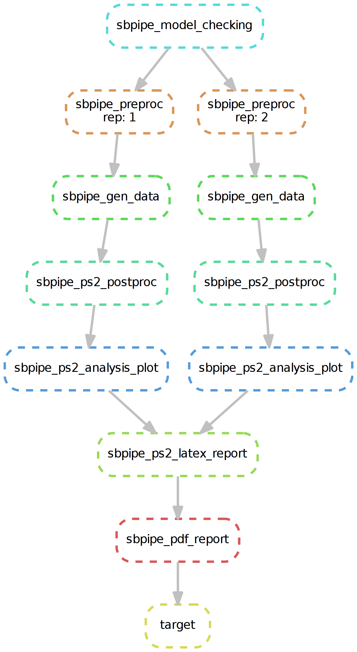
Snakemake workflow for SBpipe pipeline double parameter scan
Configuration for the mathematical models
SBpipe can run COPASI models or models coded in any programming language using a Python wrapper to invoke them.
COPASI models
A COPASI model must be configured as follow using the command
CopasiUI:
pipeline: simulation
- Tick the flag executable in the Time Course Task.
- Select a report template for the Time Course Task.
- Save the report in the same folder with the same name as the model but replacing the extension .cps with .csv (extensions .txt, .tsv, or .dat are also accepted by SBpipe).
pipelines: single or double parameter scan
- Tick the flag executable in the Parameter Scan Task.
- Select a report template for the Parameter Scan Task.
- Save the report in the same folder with the same name as the model but replacing the extension .cps with .csv (extensions .txt, .tsv, or .dat are also accepted by SBpipe)
pipeline: parameter estimation
- Tick the flag executable in the Parameter Estimation Task.
- Select the report template for the Parameter Estimation Task.
- Save the report in the same folder with the same name as the model but replacing the extension .cps with .csv (extensions .txt, .tsv, or .dat are also accepted by SBpipe)
For tasks such as parameter estimation using COPASI, it is recommended
to move the data set into the folder Models/ so that the COPASI
model file and its associated experimental data files are stored in the
same folder.
Python wrapper executing models coded in any language
Users can use Python as a wrapper to execute models (programs) coded in
any programming language. The model must be functional and a Python
wrapper should be able to run it via the command python. The program
must receive the report file name as input argument (see examples in
sbpipe/tests/). If the program generates a model simulation, a report
file must be generated including the column Time. Report fields must
be separated by TAB, and row names must be discarded. If the program
runs a parameter estimation, a report file must be generated including
the objective value as first column column, and the estimated parameters
as following columns. Rows are the evaluated functions. Report fields
must be separated by TAB, and row names must be discarded.
The following example illustrates how SBpipe can simulate a model called
sde_periodic_drift.r and coded in R, using a Python wrapper called
sde_periodic_drift.py. Both the Python wrapper and R model are
stored in the folder Models/. The idea is that the configuration
file tells SBpipe to run the Python wrapper which receives the report
file name as input argument and forwards it to the R model. After
executing, the results are stored in this report, enabling SBpipe to
analyse the results. The full example is stored in:
sbpipe/tests/r_models/.
# Configuration file invoking the Python wrapper `sde_periodic_drift.py`
# Note that simulator must be set to "Python"
generate_data: True
analyse_data: True
generate_report: True
project_dir: "."
simulator: "Python"
model: "sde_periodic_drift.py"
cluster: "local"
local_cpus: 7
runs: 14
exp_dataset: ""
plot_exp_dataset: False
exp_dataset_alpha: 1.0
xaxis_label: "Time"
yaxis_label: "#"
# Python wrapper: `sde_periodic_drift.py`.

import os
import sys
import subprocess
import shlex

# This is a Python wrapper used to run an R model.
# The R model receives the report_filename as input
# and must add the results to it.

# Retrieve the report file name
report_filename = "sde_periodic_drift.csv"
if len(sys.argv) > 1:
    report_filename = sys.argv[1]

command = 'Rscript --vanilla ' + \
          os.path.join(os.path.dirname(__file__), 'sde_periodic_drift.r') + \
          ' ' + report_filename

# Block until command is finished
subprocess.call(shlex.split(command))
# R model `sde_periodic_drift.r`

# Model from https://cran.r-project.org/web/packages/sde/sde.pdf

# import sde package
# sde and its dependencies must be installed.
if(!require(sde)){
    install.packages('sde')
    library(sde)
}

# Retrieve the report file name (necessary for stochastic simulations)
args <- commandArgs(trailingOnly=TRUE)
report_filename = "sde_periodic_drift.csv"
if(length(args) > 0) {
    report_filename <- args[1]
}


# Model definition
# ---------------------------------------------
# set.seed()
d <- expression(sin(x))
d.x <- expression(cos(x))
A <- function(x) 1-cos(x)

X0 <- 0
delta <- 1/20
N <- 500
time <- seq(X0, N*delta, by=delta)

# EA = exact method
periodic_drift <- sde.sim(method="EA", delta=delta, X0=X0, N=N, drift=d, drift.x=d.x, A=A)

out <- data.frame(time, periodic_drift)
# ---------------------------------------------

# Write the output. The output file must be the model name with csv or txt extension.
# Fields must be separated by TAB, and row names must be discarded.
write.table(out, file=report_filename, sep="\t", row.names=FALSE)